


Ergodicity#
This is both the most abstract page on the site and the one on which every concrete number depends. The question it answers sounds like a riddle: how can a bet with positive expectancy ruin almost everyone who plays it? The answer lies in a word borrowed from statistical physics — ergodicity — and in the distinction, simple and vertiginous, between the average computed across scenarios and the average computed across time.
Peters’s game#
The canonical example (made famous by Ole Peters) is a coin: heads, your capital is multiplied by 1.5; tails, by 0.6. The expectancy of a single toss is splendid: 0.5 × 1.5 + 0.5 × 0.6 = 1.05, an expected +5% per toss. Yet whoever plays repeatedly, reinvesting everything, ends up almost surely ruined. The trick becomes visible looking at two balanced tosses: one heads and one tails give 1.5 × 0.6 = 0.9. The median player loses 10% every two tosses, and in the long run capital grows at the geometric rate √(1.5 × 0.6) − 1 ≈ −5% per toss. How does that square with the expected +5%? The expectation is dominated by ever more improbable and ever richer trajectories: the lucky one who hits twenty heads in a row holds an astronomical sum that keeps the ensemble average high, while almost every individual trajectory slides toward zero.
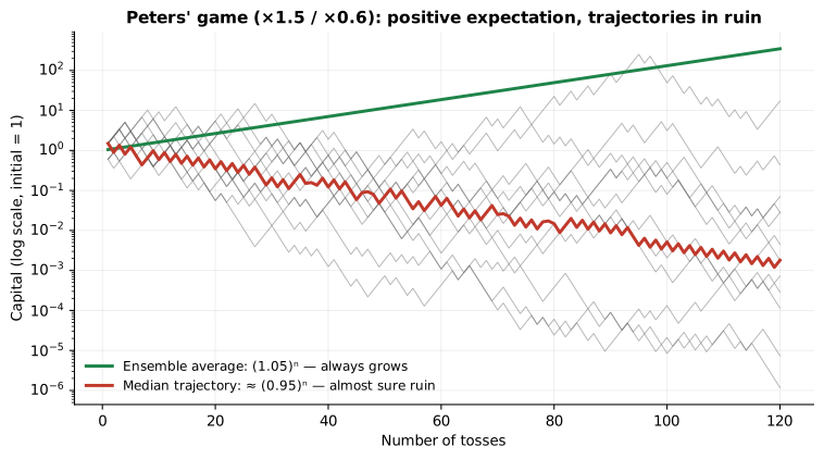
Three hundred simulated players: the ensemble average (green) grows 5% per toss, the median trajectory (red) loses 5% per toss. You are a grey line, not the green one.
Here is the heart of the matter. The ensemble average answers the question: if a thousand people play once, how much do they earn on average? The time average answers: if one person plays a thousand times, at what rate does their capital grow? A process is ergodic when the two coincide. Additive processes (you win or lose fixed amounts, independent of your capital) are. Multiplicative processes — and investing is multiplicative: returns compound on current capital — are not. You are not the ensemble: you are a single trajectory, and you live in the time average. Expectancy, by itself, is not about you.
The mathematics of the difference is well known: for multiplicative returns the long-run growth rate is approximately g ≈ μ − σ²/2, where μ is the arithmetic expected return and σ the volatility. The σ²/2 term is the volatility drag: the tax that variance levies on compounding. And here leverage enters, with its cruel asymmetry: levering by L multiplies μ by L but the drag by L², so that g(L) ≈ L·μ − L²·σ²/2 is an inverted parabola. There exists an optimal leverage (the Kelly criterion: L* = μ/σ², which maximizes long-run growth), beyond which more leverage produces less growth, and past a certain point negative growth: a winning strategy, levered enough, becomes a machine for losing with certainty. When on the Derivatives page I dismissed the myth that “derivatives are dangerous” by saying the risk lies in the ratio of notional to capital, this is exactly what I meant, in quantitative form.
Two notes before applying it. First: Kelly presupposes knowing μ and σ — and practitioners know them poorly, especially σ in the tails (Tail risk page). That is why the universal practice is fractional Kelly: half or a quarter of the theoretical leverage, sacrificing little expected growth in exchange for enormous robustness to estimation errors (on the Kelly criterion page I actually work these sums out, on a concrete case). Second: the whole argument assumes the game continues. There exists, however, a state that interrupts it: ruin, the zero (or the margin call, or the point of psychological surrender), which is an absorbing state — from there nothing compounds anymore, and no future expectancy, however brilliant, has any value left. The first rule of applied ergodicity is brutal: before maximizing growth, drive the probability of touching the absorbing state to zero. And note that I wrote “point of psychological surrender” next to the margin call, because the absorbing state is not just an accounting one: for most people there is a level of drawdown beyond which they quit — positions get closed at the lows, oaths are sworn never to touch an option again — and from there, exactly as from zero, nothing compounds anymore. Your absorbing state is the higher of your broker’s and your stomach’s, and the second must be estimated with the same honesty as the first.
Volatility selling under the ergodic lens#
I now apply the lens to this site’s trade, because short vol is the perfect case study: it is the prototype of the bet with positive expectancy (the VRP, Volatility risk premium page) and a potentially disastrous time average (the graveyard on the Risk management page). The per-trade distribution — near-certain small gain, large rare loss — is multiplicatively poisonous: the σ² that enters the drag is dominated precisely by the rare loss, and leverage amplifies it quadratically. OptionSellers.com is the textbook demonstration: positive expectancy, ensemble-grade leverage, a single tail — and the trajectory ended in the absorbing state, apology video to clients included. They were not unlucky: they played the ensemble average while living, like everyone, in the time average.
And this is why the TRPS architecture is, whether or not its practitioners use this vocabulary, ergodic engineering. I pick up the central limit theorem argument: 252 nearly independent bets a year, whose average tends to a normal distribution, with the daily skewness of −2.4 washing out to −0.1 on an annual basis. The argument is correct — but it holds on condition that no single bet can be fatal. The CLT aggregates fluctuations, it does not resurrect trajectories: if one tail in 252 can wipe out the account, no theorem can help, because compounding stops. The defenses seen so far acquire their unified meaning here: the one-day maturity limits how far the world can move within a single bet; the stop limits the loss per bet in ordinary cases; and moderate leverage limits the loss even when the stop fails (the overnight gap). All three together do one single thing: they compress the tail of the individual trade until the process, from wildly multiplicative, becomes “almost additive” — many small stakes, independent relative to capital. On an almost additive process the CLT works legitimately, the time average converges to the ensemble average, and the VRP’s positive expectancy finally becomes yours. In this precise sense I answer the question left open in the introduction: a volatility selling strategy is not ergodic — it is made ergodic by sizing and risk management, or it is not at all.
The numerical test is the one already met in Tail risk, and now I can give it its proper name. Scenario: an opening gap 15% beyond the strikes, stops useless. With 3-4x leverage the loss is on the order of 30-40% of the account: excruciating, but the process continues — at that level of drawdown you need “only” 50-65% returns to recover, feasible in a few years of premiums. With 10x leverage the loss exceeds 100%: absorbing state, end of the trajectory. The frontier between the two leverages is not a shade of aggressiveness: it is the frontier between a process that has a time average and one that does not. And it is the reason why, to the question “why not lever up a strategy with an IR of 9 even more?”, the correct answer is not prudential but mathematical.
It is worth internalizing the arithmetic of recovery too, because it is the everyday face of non-ergodicity: losses and gains are not symmetric in a multiplicative process. To get back to even after a −10% you need +11%; after a −25%, +33%; after a −50%, +100%; after a −75%, +300%. The curve is convex and accelerates: each additional point of drawdown costs more than a point of recovery, and that is why two strategies with the same arithmetic expectancy but different maximum drawdowns have different compound growth rates — the one that loses less at the worst moments finishes ahead, even while earning less at the best ones. When on the TRPS vs DHCS page I compare TRPS and DHCS on drawdown and not just on alpha, it will be this arithmetic acting as judge.
Three operating rules#
I distill the page into three rules, which are the foundation of the parameters in the Strategies section.
First: size on the worst case, not the expected one. Leverage is chosen starting from the plausible extreme scenario (the gap that jumps the stops) and requiring that the resulting loss leave the account alive and the pilot lucid. Only afterwards do you check that the expected return justifies the bother. Note the consonance with Israelov (Risk measures page): sizing on a stress-test loss budget is exactly this principle in institutional form — and its corollary, alpha scaling linearly with the tail budget, is the financial version of the ergodic theorem: return is bought by paying in potential ruin risk, at a known tariff.
Second: protect the compounding, not the individual trade. Small, frequent losses (the “false alarm” stops that irritate so much) are the insurance premium you pay to keep the per-trade tail limited. The P&L should be judged over the year, not over the single day: it is the logic of the TRPS’s PCR, which serenely accepts a 50-60% capture on the noisiest legs.
Third: remember what you are maximizing. Not the expectancy — that belongs to the ensemble, to a god who plays all scenarios in parallel. You maximize the growth rate of your one and only trajectory, which rewards survival above all else. “To win you must first survive” is not a motivational proverb: it is the informal statement of a theorem.
The principle alone, though, is not enough: it demands numbers. The next page (Kelly criterion) takes the criterion stated here and puts it to work on a concrete case — how many puts to sell, at what leverage, at what probability of halving — with a few surprises the L* = μ/σ² formula, on its own, would never have confessed.