


Kelly criterion#
The Ergodicity page established the principle: you maximize the growth rate of your one and only trajectory, and the optimal leverage exists and is computable. This page does what the previous one only promised: the math. The question is the one every put seller re-asks before every order, and that the intuitive answers (“whatever margin allows”, “whatever lets me sleep”) never really settle: how many contracts? There is a mathematical answer, and it is seventy years old: the Kelly criterion, born at Bell Labs in 1956 and collected — theorems, applications and objections — in the MacLean, Thorp and Ziemba anthology you’ll find in the Resources, 883 pages co-edited by the man who actually used that formula for a lifetime.
The exercise that follows applies that framework to a deliberately very defensive configuration of the house strategy: SPX puts at 5% out-of-the-money, one day to expiry, the realm of 1-2 delta where the put expires worthless more than 99.9% of the time. It looks like the safest place in the world. The numbers will say something subtler — and in some ways more uncomfortable than the aggressive version. One honest premise before starting: this is an exercise, not a recommended size; the market numbers are stylized but plausible assumptions, and anyone wanting to replicate the analysis must recalibrate it on their own data, costs and constraints.
Kelly in three minutes#
The idea, already met: at every bet you invest the fraction of capital that maximizes the compound growth rate of wealth — the expected value of the logarithm of capital, not the expected profit (which would lead you to bet everything, always, all the way to certain ruin) nor minimum risk (which would lead you to bet nothing). For the simplest bet — you win b for every euro staked with probability p, you lose the stake with probability q = 1 − p — the optimal fraction has a celebrated formula: f* = (b·p − q) / b, the edge divided by the odds. A biased coin that wins 53% of the time at even odds: f* = 0.53 − 0.47 = 6% of capital on every flip. No more, no less. Breiman’s theorems (1961) guarantee that whoever bets this way ends up, with probability tending to 1, richer than anyone using any “essentially different” strategy.
Three warnings though, all documented in the anthology and all decisive for what follows.
First: the famous formula only holds for binary bets. For multi-outcome payoffs you must go back to the definition and numerically maximize g(f) = E[ln(1 + f·X)], where X is the payoff per unit invested; and if the bet can lose more than the stake — short sales, futures, sold options: our case — Thorp’s generalization for “win b with probability p, lose a with probability q” is f* = (b·p − a·q) / (a·b).
Second: full Kelly is violent. An illuminating formula (Thorp attributes it to Don Schlesinger) gives the probability that capital ever falls below a fraction x of its starting value, when you bet a fraction c of the optimal Kelly: P = x^(2/c − 1). At full Kelly (c = 1) the exponent is 1: the probability of ever halving your capital is 50%; of seeing it cut to a tenth, 10%. At half Kelly the exponent becomes 3 and the halving probability collapses to 12.5%, sacrificing only a quarter of the growth — relative growth is c·(2 − c): at half Kelly, 75%.
Third: erring on the high side is fatal, on the low side venial. The growth curve is the hill of the Ergodicity page: flat near the top, precipitous beyond; at twice the optimal Kelly growth returns to zero (there is an elegant proof by Markowitz in the anthology), beyond that it turns negative — you head toward ruin while winning on average every single bet. And the Chopra-Ziemba study (1993) adds the cruel detail: estimation errors on the mean cost about twenty times those on the variance, and the ratio worsens precisely for aggressive bettors. The input you will almost certainly get wrong is exactly the one that does the most damage, and the damage is asymmetric toward overbetting. Hence the book’s unanimous rule, which in Ergodicity I called fractional Kelly: estimate the edge pessimistically and bet half or a quarter of the computed Kelly.
The inverted payoff and the no-ruin ceiling#
Selling OTM 1DTE puts is Kelly’s anti-bet: you almost always win a tiny amount and rarely lose a potentially enormous one. And the farther the strike, the smaller the coins and the faster the steamroller is already going when it arrives. The criterion has no prejudice about the sign of skewness — but you must feed it the true payoff, tails included.
I formalize the bare minimum. X is the P&L in dollars per contract at expiry (premium received minus any intrinsic value, times 100); the sizing variable is ν = N/W, contracts per dollar of capital; the optimal Kelly solves E[X / (1 + ν·X)] = 0. Two derived quantities make everything readable: the notional leverage (strike × 100 × contracts / capital — the number from the Capital efficiency page) and the worst-case loss relative to capital.
And here, before optimizing anything, Kelly delivers its first result. The logarithm of a negative number does not exist: the very domain of the problem requires that the worst-case loss not exceed the capital. The theoretical maximum number of contracts is capital divided by the worst-case loss per contract. With SPX at 7,500, a 5% OTM strike (7,125) and a worst-case scenario of −20% overnight — October 19, 1987 did −20.5%: not science fiction, it is the historical record from the Tail risk page — the loss per contract is 100 × [(20% − 5%) × 7,500] minus the premium: about $112,460. A one-million account cannot sell more than 1,000,000 / 112,460 = 8.89 contracts — notional leverage 6.3× — even wanting to maximize growth with no regard for risk whatsoever. Whoever sells more is not making an aggressive bet: they are making a bet that the mathematics of compound growth classifies as certain ruin, if repeated.
The model: four scenarios with honest tails#
Thorp insists on a point practitioners happily skip: for non-binary payoffs mean and variance are not enough — you need the whole distribution. And for the S&P 500 the tails are those of the Tail risk page: a daily decline beyond 5% would be, for a Gaussian with volatility around 1%, a once-in-a-few-million-years event; in reality it has happened about fifteen times since 1950 — roughly one session in a thousand — concentrated in a few cursed weeks (October 1987, October 2008, March 2020).
So I build a four-state model, deliberately simple but with the tails in the right place. Parameters: capital $1,000,000, SPX at 7,500, strike 7,125, premium 0.40 points = $40 per contract (stylized: a 1DTE that far out quotes a few tenths of a point, more in high-volatility regimes).
| Scenario | Probability | SPX return in 1 day | P&L per contract |
|---|---|---|---|
| The put expires worthless | 99.90% | better than −5% | +$40 |
| Moderate breach | 0.06% | about −6% | −$7,460 |
| Severe decline | 0.03% | about −9% | −$29,960 |
| Extreme (1987-style) | 0.01% | about −20% | −$112,460 |
The losses are all computed the same way: 100 × [(decline − 5%) × 7,500] minus the premium. The expected value that comes out is +$15.25 per contract: about 38% of the premium received is net edge, the rest is the actuarial cost of the tails. It is the volatility risk premium in miniature, and it is the reason the strategy can make sense. But look at the rest of the ID card: standard deviation $1,253 — 82 times the mean — and skewness −77: the farther the strike, the more the distribution deforms — moving the strike away does not tame the monster, it concentrates it.
The trap: mean-variance Kelly prescribes ruin#
On the Ergodicity page I quoted the continuous version of the criterion, L* = μ/σ² — the one Thorp uses to compute that the theoretical Kelly on the historical S&P 500 is 2.2× leverage, adding immediately that using it would be insane because prices jump. Let’s apply it, to see the effect, to our strategy’s P&L series (mean $15.25, variance 1.57 million): out come 9.7 contracts per million.
Re-read the ceiling paragraph: the absolute maximum was 8.89. Mean-variance Kelly — the “textbook” formula — prescribes more contracts than the limit beyond which the 1987 scenario wipes out the account and sends it into debt. It is not aggressive sizing: it is certain ruin dressed up as optimization, and no alarm would ring, because mean and variance are blindly satisfied with their snapshot of the risk. With a skewness of −77, the moments beyond the second — which the formula ignores — are not a correction: they are the substance. The formula from Ergodicity holds for well-behaved processes; on this payoff it is an order of self-destruction.
Rule to pin above the monitor: never size a short volatility strategy with mean-variance formulas — always discrete scenarios, with the tails calibrated on the distribution the data actually show: the cubic law. And the farther OTM the strike, the more vital the rule: here the textbook formula does not merely inflate the sizing, it pushes it past the bankruptcy threshold. If it is any consolation, it is conceptually the same mistake that sank Long-Term Capital Management: elegant models on the first two moments, real tails on the account.
What is the cubic law? The most solid empirical law we have about market tails: the probability of a decline beyond a threshold x decays as x^−3 — a power law with exponent 3, not “a Gaussian with somewhat fat tails”. It was documented by Gabaix, Gopikrishnan, Plerou and Stanley on roughly one billion observations: it holds from 15-minute to weekly horizons, across large and small stocks, across decades and across markets (S&P 500, Nikkei, Hang-Seng: exponents between 3.0 and 3.3), and it is the precision measurement of that “3-4” of Bouchaud and Potters already met on the Tail risk page — Bouchaud, who turned this idea into a program: you size against the power-law tail, not against the bell curve. The detail that concerns us: crashes are not outliers to the law. On the Dow since 1925, the −20.5% of 1987 is statistically compatible with the same straight line that describes every week’s fluctuations: the cubic law prices it, the Gaussian does not. Which welds the model’s −20% scenario into place: not science fiction, extrapolation. And the extrapolation can be done by hand: under the cubic law a decline beyond 20% is (5/20)³ = 1/64 as frequent as one beyond 5% — the four-state model assigns the extreme 1/10 of the breaches, which makes it even more pessimistic than the law: deliberate prudence, given the Chopra-Ziemba lesson. With exponent 3, finally, the variance still exists but the kurtosis is infinite: any metric built on the first two moments is blind by construction, not by bad luck. To learn how to estimate tails like these without being fooled by the sample, the manual is The Fundamentals of Heavy Tails by Nair, Wierman and Zwart, in the Resources.
Exact Kelly, line by line#
Solving the optimality condition numerically (the problem is concave, the solution unique: a bisection does the job in a spreadsheet) the full picture comes out:
| Kelly fraction | Contracts per $1M | Notional leverage | Loss in the −20% scenario | Annual growth (252 trades) | P(drawdown ≥ 50%) | P(drawdown ≥ 20%) |
|---|---|---|---|---|---|---|
| Full Kelly | 4.86 | 3.46× | 54.6% | 1.15% | 50% | 80% |
| 1/2 Kelly | 2.43 | 1.73× | 27.3% | 0.79% | 12.5% | 51% |
| 1/4 Kelly | 1.21 | 0.87× | 13.7% | 0.44% | 0.8% | 21% |
| 1/8 Kelly | 0.61 | 0.43× | 6.8% | 0.23% | nearly 0% | 3.5% |
(The drawdown probabilities use the formula x^(2/c − 1); with overnight gaps they should be read as lower bounds. Growth is the compound rate above the collateral’s return: the T-bills serving as margin keep earning their own — this is the additional slice from selling puts.)
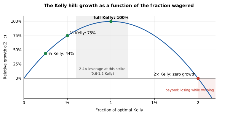
The Kelly hill: relative growth as a function of the fraction wagered. Flat near the top — half Kelly keeps 75% of the growth — and precipitous beyond: at twice Kelly growth is zero, farther out you lose while winning. Numbers from the four-scenario model.
Four lessons, in order of importance.
Lesson 1: full Kelly is half the ceiling, and still unsustainable. Exact Kelly (4.86 contracts, 3.5× leverage) sits well below the no-ruin ceiling: the math knows the 1987 scenario exists and keeps its distance. But “optimal for growth” still does not mean “sensible”: at full Kelly the wrong night costs 55% of the account in one blow, and the probability of ever halving remains a coin flip. Full Kelly is the upper frontier of rational sizing, not the advice.
Lesson 2, the most important: at 5% OTM the “blogger” leverage is a much higher Kelly fraction than it looks. The ERN method and practitioners document notional leverage between 2 and 3×; this site’s architecture, on the Capital efficiency page, speaks of 3-4×. On closer strikes, where the premium is richer, the same leverages would correspond to more prudent Kelly fractions; here, with the strike at 5%, full Kelly IS 3.5×: a 2-4× leverage corresponds to 0.6-1.2 of full Kelly — with halving probabilities from 25% up. Same leverage, risk in Kelly terms more than doubled. The reason is structural: moving the strike away, the premium (and the edge) thins out faster than the tail loss does, so the optimal Kelly in leverage terms falls. The differences between this naked model and the real strategy — active intraday stops, a strike distance revised with the VIX (the real strategy does not hold the 5% fixed: in agitated regimes the strike moves farther out), collateral that cushions — shift the numbers, but not the moral: “I win 99.9% of the time” and “I am betting little” are independent statements, and the second must be checked against Kelly, not against the win rate.
Lesson 3: halving the contracts costs little and buys a lot. From full to half Kelly, growth falls from 1.15% to 0.79% — 36 basis points a year of toll — but the halving probability collapses from 50% to 12.5% and the worst-case loss from 55% to 27%. At these magnitudes of edge, the fractional insurance costs pennies.
Lesson 4: look how small the premium pot is. At half Kelly (2.43 contracts) you collect roughly $24,500 gross a year per million, of which — if the model is right — only about $9,300 is expected edge: less than 1% a year above the collateral, before slippage and surprises. The 5% OTM version of the strategy is not the safe version: it is the small version. The bulk of the return practitioners document comes from the collateral and from closer strikes; whoever expects 10% a year selling 1 delta is either running full-Kelly-plus leverage, or dreaming.
And if the edge were half?#
The model’s most fragile input is the edge: $15.25 per contract is an estimate, and — Chopra-Ziemba teach — it is the input whose error costs twenty times the others. At these levels, moreover, hard costs are not rounding: $1.50-2 of commissions per contract are already 10-13% of the theoretical edge, before bid-ask slippage.
So I redid the numbers under a hostile scenario: same losses, tail probabilities nudged up just enough to halve the edge (from $15.25 to $7.75 per contract — the kind of error a backtest over ten lucky years commits effortlessly), while keeping the sizings computed on the optimistic parameters. Result: full Kelly grows at −0.09% — negative; half Kelly stays at +0.27% and becomes the best of the group; quarter Kelly at +0.19%. Full Kelly computed on too-optimistic parameters does not “earn less”: it destroys wealth, while winning 99.9% of the evenings. It is the numerical confirmation of the anthology’s rule, which Thorp draws in a memorable chart: if the true mean is half the estimated one, whoever uses the estimated full Kelly ends at zero growth or below, whoever uses the estimated half Kelly ends near the true optimum. With uncertain parameters, fractional is not just more prudent: it is more profitable.
What the base model does not see#
Overnight gaps#
A 1DTE spends a whole night exposed with no defenses: the stop is an intraday tool, the damage arrives with markets closed. Two formal consequences. First: drawdown formulas like x^(2/c − 1) hold for continuous processes — with jumps, capital can leap over the barriers instead of crossing them, so the true probabilities are worse than tabulated. Second: the famous property “the Kelly bettor never risks ruin” decays; with jumps, the only true safety limit is the structural ceiling. The alternative the framework makes assessable: buy an even farther OTM put and turn the naked sale into a credit spread. A 7125/6750 spread (width 375 points, assumed net premium $25) truncates the maximum loss to about $37,475 per contract: the no-ruin ceiling rises from 8.9 to 26.7 contracts per million and the optimal Kelly moves up. If the cost of protection is below the actuarial value of the tail removed, the spread dominates; often it is not — but the beauty of Kelly is that it makes the two alternatives commensurable on a single metric, the growth rate.
Margins: here, surprise, they do not bite first#
With Reg-T margin on index options (about 15% of the underlying minus the OTM amount, plus the premium), one contract of the example ties up about $75,000. Full Kelly requires $365,000 per million (36% of equity), half Kelly $182,000 (18%). Unlike the close-strike configuration — where margin saturates the account before Kelly says stop — here Kelly is the binding constraint, not the broker. It is a less innocent observation than it looks: at 5% OTM the margin would let you sell 12-13 contracts, well beyond the ruin ceiling. The broker’s margin protects him, not your compound growth. The prudential rule of the Capital efficiency page stays valid: size so that post-stress margin remains below half of post-loss equity.
Clustered losses and the post-crash temptation#
The 1DTE sales from Monday to Friday — five a week — are not independent bets: in crash regimes losses arrive in sequence, with correlation tending to 1 — and for a 5% strike this is particularly true, because breaches only occur in extreme regimes, where the bad days come one after another (March 2020: three potential breaches in six sessions). Here, though, the model — which keeps the strike nailed to 5% — is harsher than the real strategy: the OTM distance re-anchors to the VIX at every sale, and after the first bad day the following strikes move farther out — the cluster does not vanish, but it thins (the first day’s gap, that one, stays whole). The anthology treats the case of simultaneous correlated bets and the moral is blunt: sizing must be computed on the cumulative risk of the cluster, not the single day. If a typical crash lasts 3-5 sessions, the effective capital at risk is 3-5 times that of the single trade: it is equivalent to further dividing the fraction by 2-3.
And then there is Proebsting’s paradox, a gem that seems written for volatility sellers. Todd Proebsting asked Thorp: if Kelly tells me to bet 25% at 2:1 odds, and then someone offers me 5:1 on the same bet, how much do I add? Kelly’s correct answer: another 22.5% — 47.5% total, more than the 40% Kelly would have prescribed for the 5:1 odds alone. Iterating with ever-better odds, the cumulative fraction tends to 1: applying Kelly sequentially to ever-nicer opportunities on the same exposure leads to ruin, even though every single step is formally optimal. The short-vol translation is chilling: after a loss the VIX explodes, 5% OTM premiums increase tenfold, and Kelly recomputed on the new capital can suggest more contracts than before — a martingale dressed up as optimization. The rule that follows: after tail losses, first update the conditional probabilities (which have worsened), then recompute the sizing. Never increase the contracts just because the premium went up.
Bonus: fix the risk, derive the contracts#
The drawdown formula can be used in reverse, and it is perhaps its most practical use. Decide the risk you tolerate — say: probability of halving no more than 5% — and solve for the fraction: x^(2/c − 1) = 0.05 with x = 0.5 gives c ≈ 0.376. In our model: 0.376 × 4.86 = 1.83 contracts per million, 1.30× leverage. Whoever tolerates no more than a one-in-twenty chance of halving must stay under two contracts per million on this strike. It is the kind of number no intuition produces on its own.
The case for the prosecution#
An honest page must give the prosecution its say. The anthology holds at least four arguments that shrink — or question — the whole enterprise, and on the 5% OTM configuration they hit even harder.
First: Kelly can answer “zero”. The criterion presupposes a known positive edge. Here the edge is $15 gross per contract — an estimate thin as a razor, which two dollars of commissions and a little slippage cut by 15-25% before the model is even debated. If the true net premium, after costs and honest tails, were zero, the optimal Kelly is zero contracts. That is not a failure of the framework: it is one of its legitimate answers, and the farther the strike, the more probable that answer.
Second: Samuelson’s objection counts double for whoever decumulates. Paul Samuelson, the criterion’s historic critic, spent decades repeating — once even in an article written entirely in one-syllable words — that maximizing growth does not equal maximizing your utility. The anthology concedes the point: whoever has risk aversion greater than logarithmic must stay below Kelly, and no long horizon saves them. This strategy’s typical audience — someone living off the portfolio — has a steeply rising marginal utility in the severe-drawdown zone: their subjective optimum is closer to one-eighth Kelly (half a contract per million!) than to one-half.
Third: the track record proves nothing for years — here, for decades. With one breach every thousand sessions it takes four years just to observe one loss event on average. A five-year backtest can literally contain no tail at all: a 99.9% win rate is compatible both with a true edge and with a masked negative one — the sample problem of the Tail risk page, raised to a power. The anthology holds a chilling example on the slowness of inference: to distinguish with 84% confidence two games with 1.0% and 1.1% edge you need two million trials. For a strategy whose informative events arrive once every four years, serious statistics is done on the tails implied in prices and on the index’s long history, not on your own P&L.
Fourth: behavioral risk is part of the model. The anthology’s simulations — seven hundred consecutive bets, all with a 14% advantage — show that full Kelly can still turn $1,000 into $4, and that no fraction eliminates long losing streaks. For a strategy whose edge concentrates after crashes, when premiums are rich, quitting at the bottom — the standard human reaction, the psychological absorbing state of the Ergodicity page — means collecting all the tails and missing all the recoveries. Overbetting is not paid only in money: it is paid in the probability of quitting at the worst moment.
The takeaway#
- The absolute ceiling is capital divided by the worst-case loss: with 5% OTM puts on SPX 7,500 and a −20% scenario, 8.9 contracts per million (6.3× leverage). Above that, it is not trading: it is deferred ruin.
- Mean-variance Kelly here prescribes 9.7 contracts — beyond the ruin ceiling. With skewness −77 the μ/σ² formula is not an imprecise approximation: it is an order of self-destruction. Discrete scenarios with the tails inside, only.
- Honest full Kelly is 4.86 contracts (3.5× leverage) with expected growth of barely 1.15% a year above the collateral — and it turns negative if the estimated edge is twice the true one. The sensible zone is a quarter-to-half Kelly: 1.2-2.4 contracts per million, 0.9-1.7× leverage, with the worst-case cap and a further cut for loss clustering.
- At 5% OTM the practitioners’ 2-4× leverage is not prudent: it is 0.6-1.2 of full Kelly, far more aggressive — in Kelly terms — than the same leverage on closer strikes. A 99.9% win rate does not measure how much you are betting; Kelly does.
- The realistic return of this configuration is a few tenths of a point above the collateral: the deep-OTM version is not the safe version of the strategy, it is the small one. If the numbers you expect are bigger, either the strike is closer (then redo these sums with more probable tails), or the leverage is full-Kelly-plus (then re-read point 3).
The true value of the Kelly criterion for a put seller is not the magic number: it is the map. Knowing that the ruin ceiling exists and is computable; knowing that the broker would let you cross it; knowing that at these strikes leverage doubles the risk without doubling the edge; knowing that the input to watch is the edge, not the win rate. The difference between whoever sells volatility with a map and whoever sells it by feel does not show in the good months: it shows the morning after the next −20%.
With this, the risk section truly closes. You now have the instruments (Derivatives section), the premium to harvest (Volatility risk premium), the right metrics (Risk measures), the map of the tails (Tail risk), the principle governing the sizing (Ergodicity) and even the sums worked out. It is time to build the Strategies.