


CTA trend following — TSMOM#
If you’ve read the pages up to here, you know a single trade by now: selling insurance. This page steps outside that perimeter, because the third strategy doesn’t sell volatility — if anything, as you’ll see, it replicates buying it. It’s a CTA trend following strategy (in its academic form: time-series momentum, TSMOM) on futures diversified across six sectors — equity indices, Treasuries, currencies, metals, energy, agriculturals — that buys markets on the way up and sells them on the way down: every trading day the bot reads the sign of each instrument’s returns over the last 1, 3 and 12 months, takes a position in the direction that comes out, sizes it in inverse proportion to volatility, and moves only when the deviation from the target exceeds a non-trading band. I keep it, live alongside the TRPS and the DHCS, because it’s their natural complement: the literature points to it as the liquid strategy that best gets through precisely the two scenarios — prolonged equity bear markets and inflationary regimes — in which options selling and the collateral portfolio suffer together. And it didn’t come out of nowhere: it’s the extension of two things the system was already doing. The first is the futures roll — the bot was already rolling contracts for the night guard and for the DHCS hedge (Futures page), and here that service function becomes the engine of a strategy in its own right. The second is the return stacking of the Capital efficiency page: futures are held on margin, so the trend premium stacks on top of the portfolio and on top of the VRP already collected, without a dollar of dedicated capital. I’ll cover the rationale, the critical side of the literature, the exact recipe, the universe, the honest expectations and the weak points, in that order.
Why trend pays#
Time-series momentum is, in all likelihood, the best-documented anomaly in the financial literature: markets that have risen over the past 1-12 months tend, on average, to keep rising; those that have fallen, to keep falling; beyond 12-24 months the signal reverses. The foundational paper by Moskowitz, Ooi and Pedersen (Time Series Momentum) measures it on 58 futures across every asset class; Babu and coauthors (Trends Everywhere) find it again on 82 markets, including ones discovered after the recipe was published, which is the most honest out-of-sample test there is; Lempérière and his CFM colleagues (Two Centuries of Trend Following) reconstruct it back to 1800 with a statistical significance — a t-stat around 10 — that has no equal in this field; Hurst, Ooi and Pedersen (A Century of Evidence on Trend-Following Investing) confirm over a century that the premium is positive in every decade, the two world wars included. It’s not a fragile pattern dug out of some corner of the data: it’s everywhere you look, and has been for two centuries.
Why should it persist? The three classic behavioral explanations — the conservatism of investors who update their beliefs too slowly (Barberis, Shleifer and Vishny, A Model of Investor Sentiment), the overconfidence that credits successes to oneself and failures to chance (Daniel, Hirshleifer and Subrahmanyam, Investor Psychology and Security Market Under- and Overreactions), the gradual diffusion of information among investors who each observe only a piece of it (Hong and Stein, A Unified Theory of Underreaction, Momentum Trading, and Overreaction) — all produce the same footprint: underreaction to news on the horizon of months, overreaction and reversal beyond the year. These are documented, stable cognitive biases, not technical inefficiencies a fast market maker could arbitrage away; and the mechanism works market by market, which makes the time-series version on a few futures the faithful transposition of the theory. To these, add a non-behavioral channel you already know: whoever hedges risks is in a hurry, whoever absorbs them gets paid — the same hedging pressures that generate the VRP push prices slowly toward the new equilibrium, and the trend follower is the ferryman who collects the toll.
Before the evidence wins you over completely, though, there’s a caveat that changes the entire design: the premium per individual market is modest — a Sharpe of 0.3-0.4, less than buying and holding equities returns — and the strategy’s value is one of aggregation. The trends of the six sectors are nearly uncorrelated with one another, and putting together fifteen or so markets multiplies the return-to-risk ratio by a factor the literature estimates between 2 and 4, depending on the breadth of the universe. The engine is not the signal: it’s the diversification.
The critical side#
If the evidence is so overwhelming, why doesn’t everyone do this — and why did most of those who tried give up? Before the recipe we need the devil’s advocate, because on this strategy the critical literature is as sharp as the celebratory kind, and the design I describe below is a child of the former more than of the latter. Huang and coauthors (Time-Series Momentum: Is It There?) show that much of the statistical significance of the foundational papers comes from the markets’ long-run drift combined with vol scaling, not from the signal itself: the countermeasure is to always compare the strategy against equivalent passive benchmarks, never against zero. Bhardwaj, Gorton and Rouwenhorst (Fooling Some of the People All of the Time) document that the gross premium of the CTA industry did exist, but the fees — the 4.5% a year of 2-and-20 — ate it whole, leaving the investor a T-bill return: the lesson, for a do-it-yourselfer, is that the absence of that fee wedge is the only structural advantage at his disposal, to be defended with low turnover and execution costs watched like a family budget. Daniel and Moskowitz (Momentum Crashes) locate momentum’s characteristic risk: the crashes arrive in the rebounds after panics, when the short leg finds itself on the wrong side of a market turning faster than the signal — the time-series version suffers it less than the cross-sectional one, but it is not immune. Ilmanen and coauthors (How Do Factor Premia Vary Over Time?) measure over a century the out-of-sample decay of factor premia: a 20-50% haircut relative to the published numbers is the honest estimate of what awaits whoever implements today, and — an even more useful verdict — every attempt at macro timing of the premia has produced negative alphas out of sample. Park and Irwin (What Do We Know About the Profitability of Technical Analysis?), finally, remind us that data snooping is the field’s occupational disease: thousands of rules tried on the same data always produce some apparent winner.
The design consequences are three, and non-negotiable: zero optimized parameters (the 1/3/12-month lookbacks are constants taken from the literature, not the result of a search on my backtest); a fixed-weight ensemble instead of the “best” lookback; no timing — no macro filters, no adaptive weights, no discretionary reductions. Every added complication is one more bet against Park and Irwin.
The recipe#
The good news is that the whole recipe fits on one page, and not out of laziness: after the critical side, every piece you see below is the simplest of its kind, by choice.
The signal. For each instrument, the cumulative return over 21, 63 and 252 trading days (roughly 1, 3 and 12 months); of each, only the sign is taken; the average of the three signs is the signal, which can be −1, −⅓, +⅓ or +1. That’s all — and the simplicity is deliberate: Levine and Pedersen (Which Trend Is Your Friend?) show that all linear forms of trend measurement (moving averages, crossovers, filters) are statistically equivalent, so you pick the one simplest to implement and test. The ensemble serves two purposes: it avoids betting on a single horizon, and it includes the short lookbacks that — this is the result of Hamill, Rattray and van Hemert (Trend Following: Equity and Bond Crisis Alpha) and of Harvey and coauthors — generate the protection in crashes, where the 12-month alone arrives systematically late.
The size. Each instrument’s target exposure is the signal multiplied by a fixed volatility budget — around 2% of the strategy’s capital per market — and divided by the instrument’s volatility, estimated with an exponentially weighted moving average of returns (60-day center of mass) and a prudential floor at half the long-run volatility, because squashed-vol regimes are exactly the ones in which you don’t want to be caught with inflated positions. Same vol, same importance: a point of risk in copper is worth a point of risk in the Nasdaq (that’s the equal-vol of Asness, Moskowitz and Pedersen, Value and Momentum Everywhere). The exposure is then rounded to whole contracts — and at retail capital the rounding is part of the design, not a detail: with a ⅓ signal many targets quantize to zero, which works as a natural non-trading band.
The band. You trade only if the deviation between target position and actual position exceeds 25% of the target, on top of the minimum granularity of one contract. It’s the household version of the result of Gârleanu and Pedersen (Dynamic Trading with Predictable Returns and Transaction Costs): with real transaction costs you never chase the exact target, you move only when the gap is worth the trip. The practical consequence: the evaluation is daily but the effective trading frequency is close to monthly, and the expected frictions stay on the order of 0.3-0.6% a year — the budget within which, by Bhardwaj’s account, the strategy must be able to survive even at double or triple the costs.
Vol targeting. Above the level of the individual instruments, a portfolio multiplier scales all positions to keep the strategy’s volatility near a target of 10% a year, with a leverage cap at 1.5: when the strategy’s realized vol rises, size comes down, and vice versa. It’s the volatility management of Barroso and Santa-Clara (Momentum Has Its Moments) and Moreira and Muir (Volatility-Managed Portfolios), which on this style halves the kurtosis and cuts precisely the tails of Daniel and Moskowitz’s momentum crashes — the only “timing” the design admits, because it has zero free parameters and a sign fixed in advance: it can only reduce.
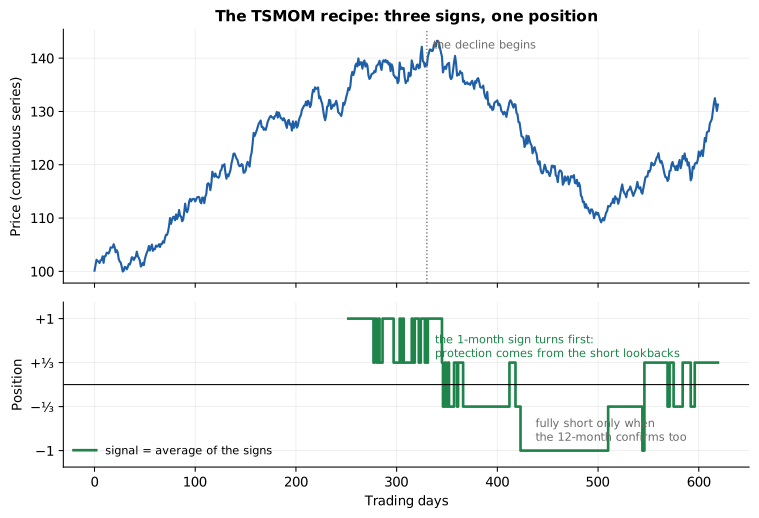
A simulated market and the mechanics of the recipe: the three signs at 1, 3 and 12 months (top) combine into the stepped position (bottom), which the vol scaling resizes and the 25% band filters. The short lookback turns first in the reversal: it’s the one that buys the protection. Illustrative numbers.
The universe: six sectors#
On which markets, then? The reference universe counts fifteen or so logical instruments: three equity indices (Nasdaq, Russell 2000, Dow), three points of the Treasury curve (2, 10 and 30 years), three currencies (euro, sterling, Australian dollar), three metals (gold, silver, copper), two energies (WTI and natural gas), two or three agriculturals (wheat, soybeans, corn). The composition chases correlations, not headcount: the rate curve is represented by its endpoints and not by the redundant middle, the soybean complex counts as a single bet, and the classes historically most generous to trend — FX, rates, commodities — weigh as much as equity, not less (Fung and Hsieh, Empirical Characteristics of Dynamic Trading Strategies; Hutchinson and O’Brien document that commodities are the only class that pays during financial crises).
The double contract size. Every logical instrument exists in two variants: the micro and the standard full-size contract (gold in tenths at $10 a point or in full lots at $100, WTI in 100-barrel micros or 1,000-barrel lots, and so on). Which family gets traded is a parameter with three modes — micro only, full only, mixed — and the choice depends on capital: at the current capital the micros are mandatory, because the volatility of a single standard contract would exceed the entire market’s risk budget on almost the whole universe, and the portfolio would collapse onto two or three positions; as capital grows the fulls become convenient (tighter spreads, lower relative commissions), and in mixed mode the migration is automatic, instrument by instrument: when a full contract’s vol fits inside the per-market budget, the bot switches to the large size, with a hysteresis that prevents ping-pong and with the family change happening only with the position closed or at the roll. The strategy is the same at $150,000 as at $3 million: only the size of the brick changes.
Two deliberate exclusions. The ES and its micro MES stay out of the universe: they are the instruments of the TRPS night guard and of the DHCS hedge, and keeping every contract assigned to a single strategy makes the position bookkeeping a trivial sum instead of a puzzle. And cryptocurrencies stay out with full cause: no support in the historical corpus, barely eight years of data, and in the test that matters — the COVID crash — bitcoin moved with the Nasdaq, adding equity beta exactly when the short puts were suffering: the opposite of the job this strategy exists to do.
At the data level, the signals run on continuous return series of the contracts held: at the roll you concatenate returns, never prices, because it’s the only way to measure what an investor would actually have pocketed — Géczy and Samonov show that momentum computed on commodity spot prices is an illusion that flips sign on rolled futures. The roll follows each market’s calendar and, on physical commodities, never crosses the first notice day: a retail trader doesn’t take delivery of barrels. The slope of the curve — the carry — gets measured and archived at every cycle, but moves no orders: the literature promotes it as a complementary signal (Koijen, Moskowitz, Pedersen and Vrugt, Carry), but its risk profile — it loses in global recessions, in all asset classes at once — is exactly what the account already owns in abundance via short puts. Trend is the complement; carry is not.
What to expect#
The honest numbers, after Ilmanen’s out-of-sample haircut: an expected net Sharpe between 0.3 and 0.5 — not the gross 1.8 of the academic backtests — with physiological drawdowns of 20-25% and, this is the hard part, possible multi-year flat stretches: the 2010-2018 decade returned trend following roughly 1% a year with the engine statistically intact (Babu and coauthors, You Can’t Always Trend When You Want — the title says it all). Whoever judges this strategy on its quarterly statement is on the wrong page; the evaluation horizon is the full cycle, and the rationale was never the Sharpe on its own: it’s what this return profile does to the rest of the portfolio, which is the subject of the next page.
And this is the configuration the system runs in now: the CTA strategy is live alongside the TRPS and the DHCS, with one cycle a day in mid-morning, size governed by the volatility budgets described here and a monthly report that reaches me by email on the first Monday of the month with the leg’s return, costs and margin (the mechanics are on The CTA bot page). As always on this site, the expected numbers are a matter of literature and record, not a promise: Disclaimers page.
The weak points#
I close with the list of what can hurt, because it’s the part no brochure puts on the cover — and the part you have to accept before, not after.
The whipsaw is the fare. In sideways markets the signal buys the local highs and sells the local lows, losing little but often: it’s the insurance premium the trend follower pays — the exact mirror image of the 15 cents the TRPS collects — in exchange for the convexity in prolonged moves. Whoever can’t tolerate long sequences of small losses won’t tolerate this strategy.
Gaps are not covered. Trend convexity lives on moves that last weeks or months; on a one-day overnight jump — the BoJ night, the Monday of 1987 — the signal has no time to turn, and the account’s protection stays with the guardrails of the Risk management section and with the TRPS’s defenses. Buying this strategy as “crash cover” is buying it for the wrong reason: it covers the prolonged declines, not the lightning bolts.
Quantization. At retail capital half the targets are worth 0 or 1 contract: the real strategy chases the theoretical one with a permanent rounding error, declared and measured. With the micros the error is tolerable; it’s still a headwind the institutional backtests don’t have.
Correlations on the bad days. Diversification across six sectors is the engine, but in risk-on/risk-off regimes correlations all rise together and portfolio vol overshoots the target exactly when you’d least want it to; Hurst and coauthors identify the average correlation across markets as the only monotone predictor of the style’s performance. Vol targeting mitigates; it doesn’t eliminate.
Abandonment is risk number one. Bhardwaj’s most merciless statistic isn’t about markets but about operators: the typical pattern of the failed CTA is recalibration after the drawdown — changing the parameters, “fixing” the signal, switching everything off at the low. That’s why the lookbacks are constants and not parameters, and every reduction rule has its sign fixed in advance: the strategy is designed to make it hard for me to perform the gesture that has historically killed its kind.
Parameter recap (plausible ranges): fixed-weight ensemble of the 1/3/12-month signs (design constants, not parameters); volatility budget per instrument of 1.5-2% of the strategy’s capital; vol estimated with a 60-day EWMA and a floor at half the long-run vol; portfolio target of roughly 10% a year with a leverage cap of 1.5; 25% non-trading band; sector caps of 25-30%; aggregate risk cap of 50% of capital in volatility; drawdown brake at 15% with a halving of the sizes. Everything else — and it’s almost everything — is waiting.
There remains the question that decides whether this page deserves to exist: why keep in the portfolio a strategy with half the Sharpe of the other two? The answer lies not in its returns but in when they arrive, and that’s the next page.